

Turning a library of aerial imagery into a natural-language-searchable knowledge base is a problem that touches every industry that relies on geospatial data — insurance, real estate, government, infrastructure, and agriculture. The traditional path requires either manual tile-by-tile inspection or training a bespoke computer vision model for each new question. Multimodal embeddings, large language model (LLM) captioning, and vector search on AWS offer a faster alternative: index once, then query using natural language.
We worked with Vexcel, an aerial imagery and geospatial data provider that operates one of the largest aerial imagery programs in the world, to evaluate embedding models, fusion strategies, caption integration, and search methods over multi-view aerial imagery. Using its own sensors and a dedicated fleet of aircraft, Vexcel collects high-resolution data across 45+ countries and territories, delivering orthomosaic imagery, oblique imagery from multiple angles, and elevation models. The data exists, and the use cases are numerous, but turning billions of pixels into answers about the real world requires a faster path.
In this post, we walk through the problem space, our architecture on Amazon Bedrock and Amazon OpenSearch Serverless, the evaluation methodology we built on OpenStreetMap ground truth, four experiments that compared embedding models, fusion strategies, captioning, and search methods, and the practical guidance you can apply when building a similar system. You’ll learn which design choices move the needle for geospatial semantic search, including why Amazon Nova Multimodal Embeddings delivered the highest F1 scores across both benchmark queries in our evaluation. The work described here evolved into Vexcel Intelligence, a searchable imagery product.
Searching millions of aerial images without per-feature training
When a customer needs to locate swimming pools in a suburb, identify road networks in a development zone, or count solar panels across a city, someone has to manually look tile-by-tile (inspecting each map tile in turn) across millions of images. The alternative is training a computer vision model for each feature, which requires labeled data, engineering time, and ongoing retraining. When the next customer wants to find warehouses with graffiti on the side (see Figure 1), they repeat the cycle. Semantic search powered by vector embeddings removes this per-feature training step and turns natural-language queries into results in seconds.
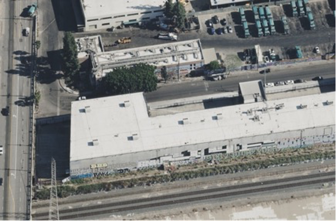
Figure 1. A typical oblique image from Vexcel, providing models rich 360-degree vision of the world
Vexcel had explored this problem through three prior POCs: an agent-based approach combining imagery with property data, a property embedding system for similarity search, and a tiled multimodal embedding pipeline with captions generated by a large language model (LLM). The third showed promise but raised key questions: which embedding model to use, how to handle multiple views per location, and whether captions actually improve results or just add cost.
The AWS Generative AI Innovation Center (GenAIIC) partnered with Vexcel to answer a focused question: what is the optimal combination of embedding model, fusion strategy, captioning approach, and search method for semantic search over multi-view aerial imagery? Vexcel brought domain expertise and real-world data, while GenAIIC contributed ML architecture, a complete ingestion-to-evaluation pipeline, and AWS service integration. The result is a system Vexcel has since evolved into Vexcel Intelligence, a product now in preview that transforms their imagery library into a searchable, AI-queryable solution.
Why geospatial imagery search is different
Geospatial imagery search is fundamentally different from searching consumer photos. A query for “swimming pool” on Google Images retrieves standalone photographs from a single perspective. Aerial imagery doesn’t work that way.
A single map tile isn’t one image. It’s seven complementary perspectives of the same location.
Each tile includes an orthophoto (the top-down RGB view), four oblique photographs captured at angles from the north, south, east, and west, a Digital Surface Model (DSM) encoding elevation including structures, and a Digital Terrain Model (DTM) representing bare ground height. The following figure shows what these seven perspectives look like for a single tile — each captures different details about the same geographic location.
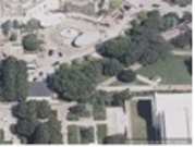

Figure 2. Seven complementary views of the same tile (top row: Ortho, North oblique, South oblique, East oblique; bottom row: West oblique, DTM, DSM)
These perspectives reveal radically different details. In the preceding figure, the building’s front façade (featuring a kiosk-like window) is only visible from the south oblique angle; the orthophoto, the remaining oblique views, and the elevation models miss it entirely. Meanwhile, the DSM captures tree canopy that obscures ground-level features in the RGB views, and the DTM strips vegetation away altogether. An embedding model that sees only one view works with incomplete information. One that sees the seven perspectives needs a strategy for combining them.
The ground truth challenge
Consumer image search has decades of labeled datasets such as ImageNet, COCO, and Open Images. Aerial feature detection at this scale has none. We needed a way to evaluate search quality without a pre-labeled corpus, which led us to OpenStreetMap as an automated ground truth source, a decision that shaped the entire evaluation framework.
Ambiguity in what counts as a correct result
The third challenge is ambiguity, and it runs deeper than view selection. Consider a search for “swimming pools” that returns a tile where the pool is visible only in the ortho photo but not in any oblique view. It is unclear whether that result is correct. The reverse case is equally ambiguous: a tile where the pool is visible from the south oblique but not from above.
Zoom level compounds this. Depending on tile resolution, a single tile might cover a city block or an entire neighborhood. In a dense suburban area, one tile could contain a dozen swimming pools. Should the ground truth require the system to return a tile if it contains a matching feature, or should it account for every instance within that tile? A tile-level match (at least one pool present) and a feature-level match (every pool accounted for) are fundamentally different evaluation criteria, and they reward different system behaviors. We had to define what “correct” means before we could measure it.
Co-designing the research agenda
Before writing a single line of optimization code, we built the evaluation harness. This was deliberate: measure before you tune. Without a rigorous way to measure search quality, every architectural decision becomes an opinion.
The engagement was structured around the following six questions, each targeting a specific architectural decision that affects search quality:
- Which embedding model best understands aerial imagery? We compared Amazon Nova Multimodal Embeddings, Amazon Titan Multimodal Embeddings G1, and Cohere Embed v4, each available in Amazon Bedrock, a fully managed service that offers a choice of high-performing foundation models (FMs) from leading AI companies through a single API. Amazon Nova, in turn, is a family of foundation models available through Amazon Bedrock.
- How should you handle seven images per geographic location? We tested per-view embeddings, late fusion (average and max-pool), LLM-weighted attention fusion, and Cohere’s native multi-image batch encoding.
- Does LLM-generated captioning improve search accuracy? We designed a custom captioning prompt that instructs the FM to analyze the seven images simultaneously as complementary views of the same geographic location, identifying each image type (ortho, oblique angles, DSM, DTM) and synthesizing a unified description across land use, built environment, infrastructure, natural features, objects, and spatial relationships. The prompt explicitly directs the model to cross-reference perspectives: when something appears unclear in one view, use other angles or elevation data to resolve it. We tested this prompt with Amazon Nova 2 Lite and Anthropic’s Claude in Amazon Bedrock, measuring whether indexing those captions alongside image embeddings improved retrieval.
- Can LLM-extracted metadata improve filtering? We used a second FM pass to extract up to 25 keyword tags from each generated caption (for example, “swimming pool”, “mature trees”, “commercial district”) and stored them in an Amazon OpenSearch Serverless text field alongside the embeddings. At query time, the same extraction runs on the user’s search query. Amazon OpenSearch Serverless k-nearest neighbor (k-NN) filtering then uses these tags as a pre-filter, narrowing the candidate set to documents whose tags match the query terms before running vector similarity. This uses native filtered k-NN to combine structured metadata with semantic search.
- Which search strategy works best for different feature types? We compared basic k-NN, multi-view fusion search, hybrid image+caption scoring, metadata-filtered search, and text-only search.
- Can you build an automated evaluation framework using publicly available ground truth? We sourced ground truth from OpenStreetMap via the Overpass API, enabling repeatable benchmarks without manual labeling.
The evaluation area was Grant Park in Chicago, with two benchmark queries: “swimming pools” (discrete object detection) and “roads” (distributed infrastructure detection). We tested approximately 100 distinct configurations across these dimensions.
Architecture overview
The system follows a five-stage pipeline (Figure 3), each stage independently swappable for A/B experimentation.
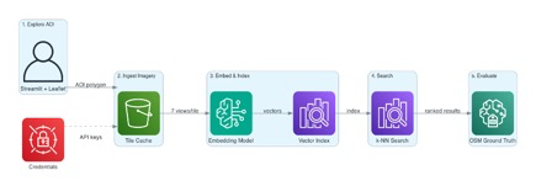
Figure 3. Five-stage pipeline architecture
Stage 1. Explore Area of Interest (AOI). Users draw a polygon on an interactive map to define their area of interest. The AOI is persisted to Amazon Simple Storage Service (Amazon S3) for reproducibility.
Stage 2. Ingest Imagery. The system fetches tiles from Vexcel’s API for every map tile intersecting the AOI at a configurable zoom level. Each tile yields up to seven images. Rate limiting (100 requests/second) and Amazon S3 caching help prevent redundant API calls. Credentials are managed through AWS Secrets Manager (Figure 4).
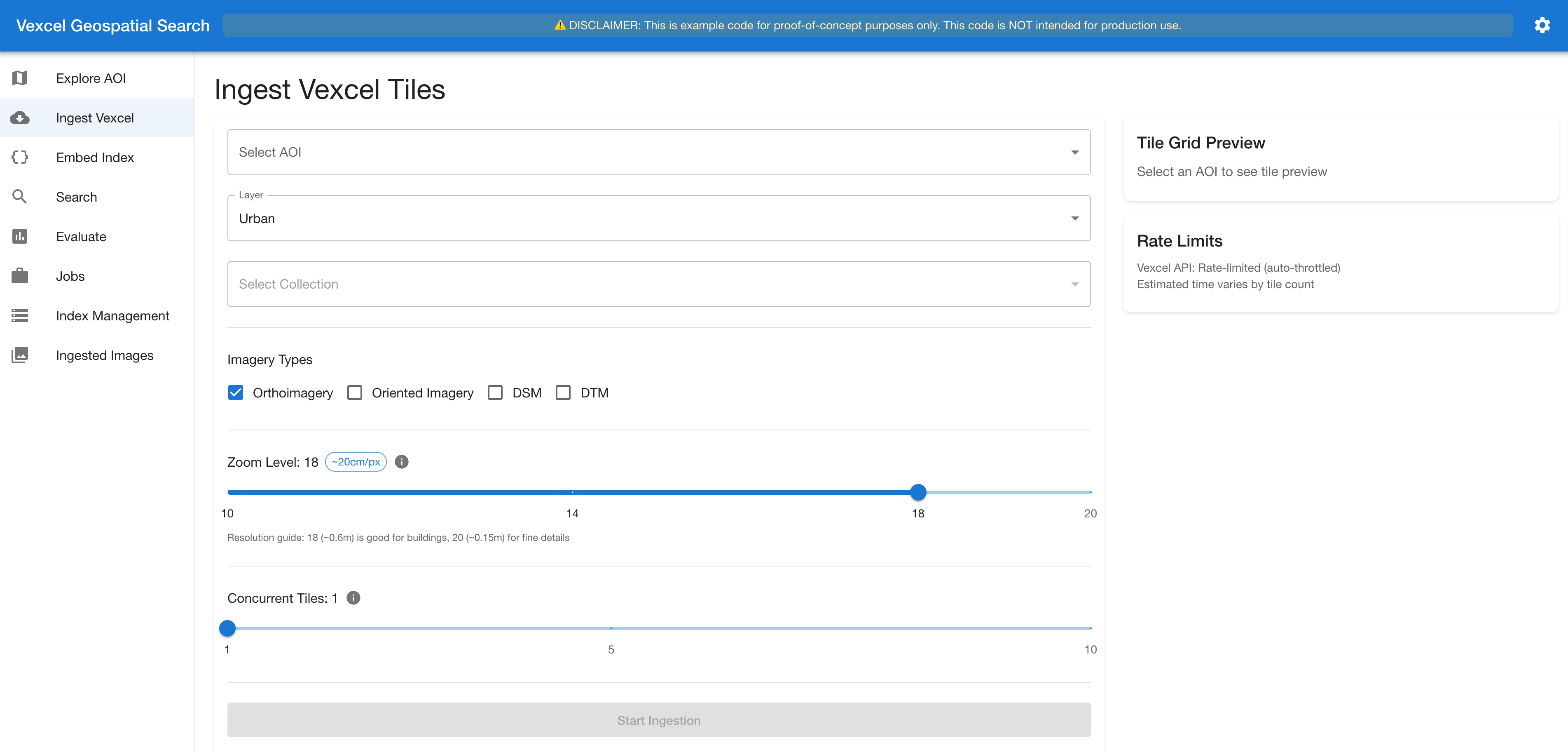
Figure 4. The ingestion interface: selecting imagery types and zoom level
Stage 3. Embed & Index. Each image passes through the selected Amazon Bedrock embedding model. Optionally, the seven views are sent to a vision LLM (Amazon Nova 2 Lite, or Anthropic’s Claude) to generate a structured text description. Embeddings and captions are then indexed into Amazon OpenSearch Serverless or Amazon S3 Vectors. The interface provides caption generation controls, a real-time dimension impact analysis, embedding model, and fusion strategy selection (Figures 5 and 6).
Stage 4. Search. Natural language queries are embedded using the same model, then matched against the index. The system auto-detects which fields exist in the index (per-view embeddings, fused embeddings, caption text, caption embeddings) and dynamically enables only the search methods that the index supports.
Stage 5. Evaluate. Search results are scored against OpenStreetMap ground truth using precision, recall, and F1 score. The evaluation framework runs the same query across every enabled search method and reports comparative metrics.
The modular design was the key architectural decision. Every component (embedding model, fusion strategy, search method, vector store) connects through a common interface. Swapping Amazon Nova Multimodal Embeddings for Cohere Embed v4 is a configuration change, not a code change. This enabled us to test ~100 configurations in hours rather than weeks.
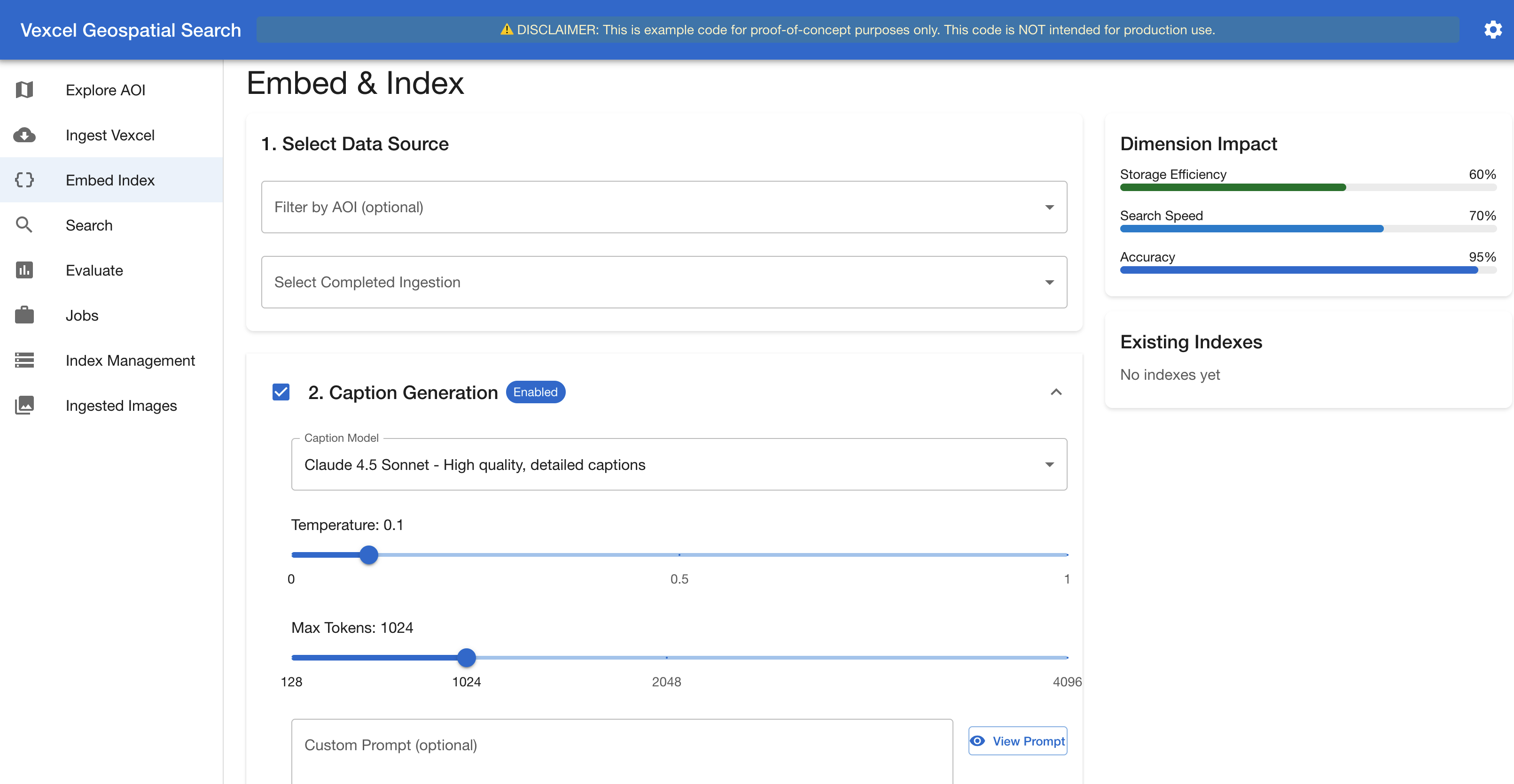
Figure 5. The Embed & Index interface – Caption Generation section
The following figure shows the embedding configuration panel, where users select the embedding model and fusion strategy for their indexing run.
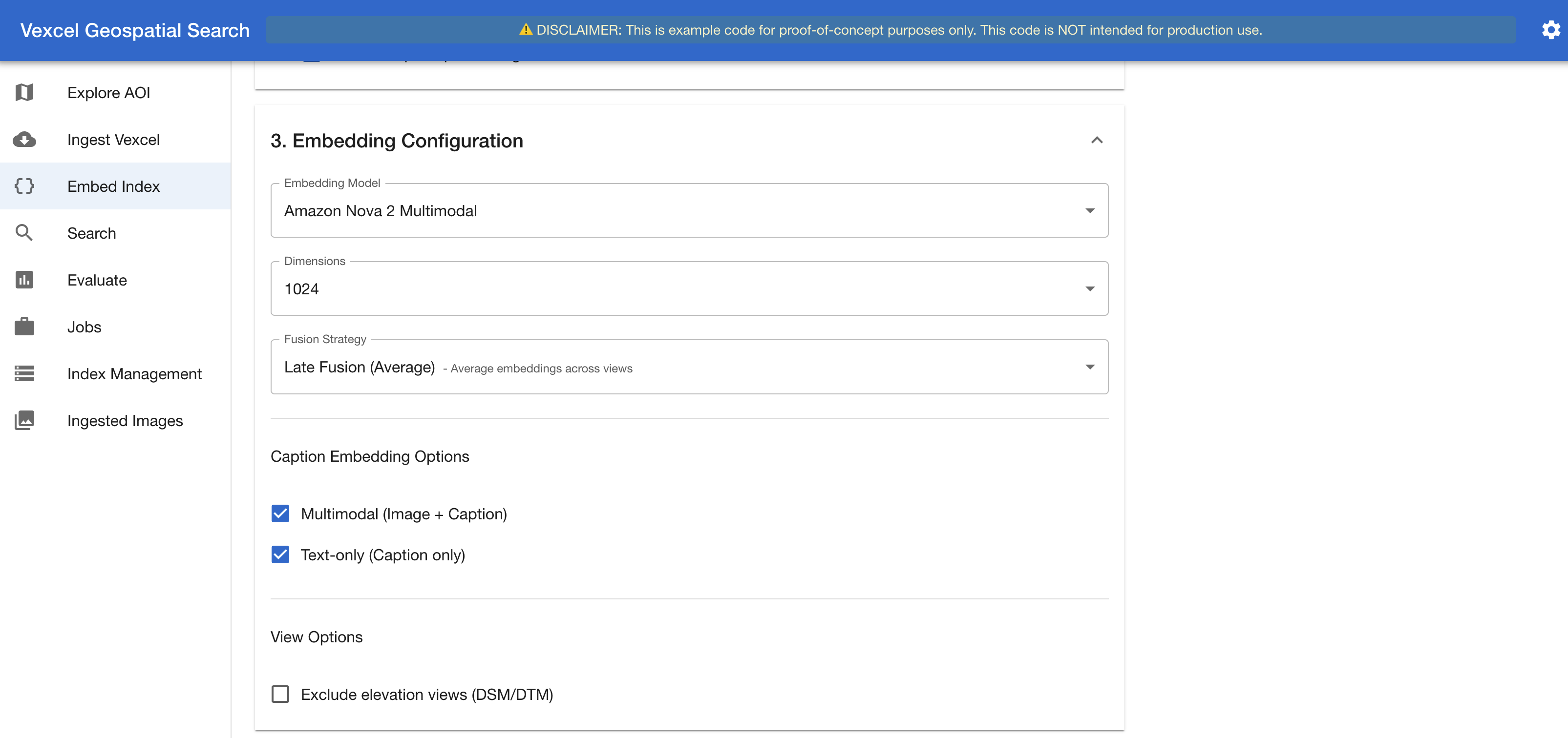
Figure 6. The Embed & Index interface – Embedding Configuration section
Choosing the right K
Every vector search returns the top k-NN results. K is a lever with real consequences, and the right value depends on how common the feature is in your dataset.
When a feature is sparse (a few swimming pools scattered across hundreds of tiles), a large K floods results with irrelevant tiles. The system retrieves K results regardless of whether K relevant tiles exist. Set K=50 when only 8 tiles contain pools, and 42 of those results are noise. Precision collapses. F1 follows.
When a feature is abundant (roads appearing in most tiles), a small K artificially caps recall. Set K=5 when 60 tiles contain roads, and you can only find 8% of them. Recall collapses. F1 score follows.
The relationship is mechanical. Precision@K = relevant_found / K. If K exceeds the number of relevant tiles, precision can never reach 1.0. Recall@K = relevant_found / total_relevant. If K is smaller than the total relevant tiles, perfect recall is impossible.
We evaluated at multiple K values simultaneously (K = 3, 5, 7, 10, 15, 20, 25, 30, 50) and tracked how precision, recall, and F1 score shifted across the range. The optimal K consistently landed near the actual count of relevant tiles in the ground truth, a number you won’t know in production. In practice, start with K=10–20 for general queries, observe the precision-recall tradeoff in your evaluation results, and adjust per feature category. The evaluation framework makes this calibration fast; rerunning with different K values costs seconds, not hours.
Two ways to measure: tile-based vs. entity-based evaluation
A single metric can mask important behavior depending on what you count as a hit. We built the evaluation framework with two complementary modes that answer different questions.
Tile-based evaluation asks: did we find the right locations? A tile is either relevant (contains at least one instance of the feature) or not. If a tile has one swimming pool or twelve, it counts as one relevant tile either way. Precision, recall, and F1 are computed over tiles.
Entity-based evaluation asks: did we find the most features? Each individual entity (each pool, each road segment) counts separately. A tile with 5 pools contributes 5 to the relevant total. Finding that tile recovers 5 entities. Missing it loses 5.
The two modes diverge when features are unevenly distributed, and in aerial imagery, they almost always are. Consider this scenario from our evaluation:
| Scenario | Tile-Based Recall | Entity-Based Recall |
| Found 1 tile with 5 pools, missed 1 tile with 1 pool (6 total) | 50% | 83% |
| Found 1 tile with 1 pool, missed 1 tile with 5 pools (6 total) | 50% | 17% |
Tile-based recall is identical in both cases: 1 of 2 tiles found. Entity-based recall reveals the critical difference: the first scenario recovered most of the actual pools; the second missed most of them.
Which mode to use depends on the question. Tile-based evaluation is the right lens when geographic coverage matters, such as “find every location that has a pool.” Entity-based evaluation matters when density matters, such as “find the areas with the most pools.” We report both because the gap between them reveals feature distribution: a large divergence signals that features are clustered in a few dense tiles rather than spread evenly across the area. The evaluation framework also computes nDCG (normalized discounted cumulative gain) using entity counts as graded relevance, and stratified metrics that break performance into sparse tiles (exactly 1 entity) versus dense tiles (2+), so you can see exactly where the system succeeds and where it struggles.
Experiment 1: Which model understands aerial imagery?
We indexed the same Grant Park dataset three times, once per embedding model, keeping other variables constant. Each model processed the same tiles, the same views, and the same Amazon OpenSearch Serverless configuration. We then ran both benchmark queries across each fusion and search configuration and computed the average F1 score per model.
Amazon Nova Multimodal Embeddings achieved the highest average F1 scores for both swimming pools (0.621) and roads (0.555) in our evaluation (Figure 7). The margin over Cohere Embed v4 was modest for swimming pools (0.621 vs. 0.606) but substantial for roads, a notable difference (0.555 vs. 0.415). Cohere Embed v4’s native multi-image batch encoding performed well for discrete objects but showed reduced sensitivity to distributed infrastructure features like road networks in our testing.
We expected Amazon Titan Multimodal Embeddings G1 to compete closely. It didn’t. Its average F1 score of 0.340 for pools was significantly lower than the Amazon Nova Multimodal Embeddings score. Worse, several configurations produced near-zero F1 scores in image-based search: cases where the model returned almost entirely irrelevant results. These weren’t outliers. They appeared consistently across specific fusion and search method combinations.
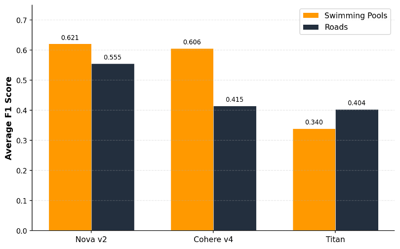
Figure 7. Average F1 score by embedding model across both benchmark queries.
The practical takeaway: model choice has an outsized effect on geospatial search quality, and the effect varies by feature type. Roads showed a meaningful performance variation across models for both feature types. If you’re starting a geospatial search project on AWS, you can default to Amazon Nova Multimodal Embeddings.
Experiment 2: How should you handle seven images per location?
Seven images per tile creates an indexing dilemma. You can store them separately (7 embeddings per tile), merge them into one (fusion), or let the model handle the combination natively.
We tested four approaches:
- Per-view embeddings: 7 separate vectors per tile, each searchable independently. Results are aggregated across views at query time.
- Late fusion (average/max-pool): Compute 7 embeddings, then average or max-pool them into a single vector. Simpler to index, but the merged vector loses view-specific signal.
- Attention fusion: An LLM assigns per-view weights based on the query, then the weighted combination produces a single embedding. A “swimming pool” query might weight the orthophoto at 0.4 while a “tall buildings” query weights the DSM at 0.35.
- Cohere batch: Cohere Embed v4’s native multi-image API processes the seven views in a single call, producing one embedding that captures cross-view relationships internally.
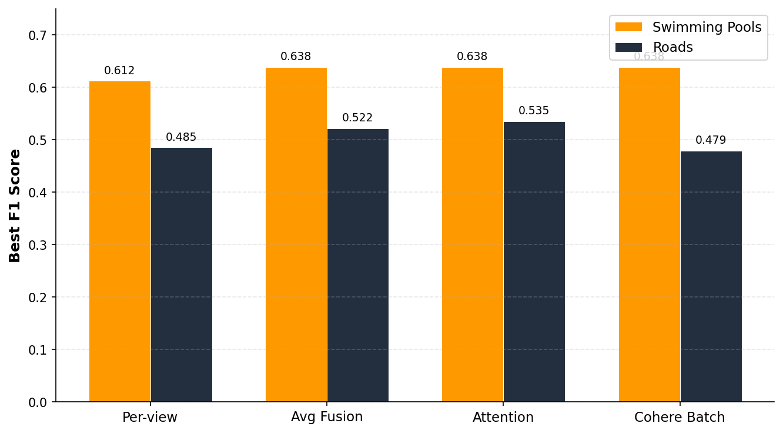
Figure 8. Best F1 score by fusion strategy across both benchmark queries.
For swimming pools, three strategies (Cohere batch, attention fusion, and late average) each achieved an average F1 score of 0.638, the highest score (Figure 8). Per-view underperformed at 0.612, largely because metadata filtering behaved inconsistently when operating across 7 separate embedding fields. The 4.2% gap between Cohere batch and per-view indicates that fusion technique choice has meaningful impact, particularly for reliability across different search methods.
For roads, the story reversed. Attention fusion led at 0.535. Late average followed at 0.522. Per-view came in at 0.485. Cohere batch dropped to 0.479, a 12% gap between best and worst. The same strategy that tied for first on pools placed last on roads.
No single fusion approach dominates across feature types. The optimal strategy depends on what you’re searching for.
Experiment 3: Does captioning help?
We used Amazon Nova 2 Lite to generate structured captions from the seven views simultaneously. The prompt instructs the model to describe land use, built environment, infrastructure, natural features, and spatial relationships visible across the full set of perspectives. The result is a single text description per tile that synthesizes information no individual view contains alone.
Caption integration turned out to be the single most impactful optimization we tested.
For swimming pools, the best Amazon Nova Multimodal Embeddings configuration with caption integration (“both methods”: image and caption embeddings fused into a combined score) achieved a best configuration F1 score of 0.638, compared to 0.573 without captions. That’s an 11% improvement. For roads, the gap was even larger: 13% (F1 of 0.555 vs. 0.490).
Here’s what surprised us: caption integration strategy mattered more than embedding model choice. Cohere Embed v4 and Amazon Nova Multimodal Embeddings achieved identical best configuration F1 scores of 0.638 for pools when paired with optimal caption integration. The captions provided a textual grounding that compensated for differences in visual embedding quality.
But captions alone aren’t enough. Text-only search (matching query terms against captions without any image embeddings) dropped 17% to F1 of 0.532 for pools. The visual signal carries information that text descriptions are missing. The best results come from combining both modalities.
Caption model choice has a measurable downstream impact. Different caption models produced different vocabularies in their descriptions, which affected downstream tag-based filtering. In some cases, one model’s captions surfaced features that another’s missed, resulting in different F1 scores for metadata-filtered search. If your pipeline uses tag-based filtering, the caption model’s vocabulary directly affects recall.
We also tested whether DSM and DTM data contributed to object detection. They didn’t. Configurations with 4 views (ortho + obliques) matched or exceeded those using the seven views including elevation. For standard object detection tasks like pools and roads, you can skip the elevation data; it adds embedding cost without improving accuracy.
Experiment 4: What is the right way to search?
We implemented five search methods (Figure 9), each representing a different tradeoff between sophistication, cost, and accuracy.
Basic k-NN: Straightforward vector similarity against the aggregated image embedding. Lowest latency, with no additional FM calls. This is the right default when captions are already baked into the index.
Image + Caption Fusion: Runs parallel k-NN searches against both the image embedding and caption embedding fields, then blends scores using a tunable alpha weight (default 0.7 image / 0.3 caption). Captures both visual and semantic similarity.
Metadata Filtering: Applies tag-based pre-filtering before vector search, narrowing the candidate set to tiles whose generated tags match the query terms. Fastest path when the user names a known feature (such as “swimming pool” or “parking lot”).
Figure 9. Search page showing the five methods with availability indicators
Text-Only Search: Keyword matching against the caption field with no vector similarity.
7-Way Imagery Fusion: Runs parallel k-NN searches across the seven per-view embedding fields plus captions, with dynamic per-query weight assignment. An FM analyzes the search query and assigns relevance weights to each view. For example, a “baseball field” query weights the orthophoto at ~0.3 for field markings, while a “multi-story buildings” query weights the DSM at ~0.35 for height data. The weighted scores are combined into a final ranking.
No single search method dominates across feature types. The optimal strategy depends on what you’re searching for, which is why the system exposes each of the five methods and the evaluation framework measures which works best per query category.
The following tables summarize search method performance for each of our two benchmark queries. For swimming pools, multiple methods achieve the same top F1 score, while roads show clearer differentiation between approaches.
Swimming pools
| Search Method | Best Config F1 | When to Use |
| Basic k-NN | 0.638 | General-purpose, low latency |
| Image + caption fusion | 0.638 | Balanced multimodal queries |
| Metadata filtering | 0.638 | High-precision object detection |
| Text-only | 0.532 | Low cost, visual features not decisive |
| 7-way imagery fusion | — | Query maps to specific view perspectives |
Roads
| Search Method | Best Config F1 | Notes |
| Basic k-NN (Nova captions) | 0.524 | Best overall for infrastructure |
| Image + caption fusion | 0.506 | Visual features dominate over caption signal |
| Text-only | 0.395 | Road descriptions too varied for pure text matching |
| Metadata filtering | 0.358 | Inconsistent tag matching on road descriptions |
Three methods tied at F1 of 0.638 for swimming pools: basic k-NN, image + caption fusion, and metadata filtering. For roads, basic k-NN dominated at 0.524. The optimal search method depends entirely on the feature type.
Metadata filtering shows the starkest contrast. It tied for best on pools because the FM extracted “swimming pool” tags that matched caption text precisely, enabling tight pre-filtering before k-NN. On roads, it collapsed to 0.358. Road descriptions in captions are more varied and less consistently tagged, making keyword pre-filtering unreliable.
The image + caption fusion approach computes a weighted combination: α × image_score + (1−α) × caption_score. We tested both manually tuned weights and FM-assigned dynamic weights. Both achieved an F1 score of 0.638 for pools. For these relatively simple queries, manual tuning sufficed. Dynamic weighting may prove more valuable for complex, multi-faceted searches where the optimal alpha varies per query; for example, “residential areas near water with commercial buildings” requires different image-vs-text weighting than “parking lots.”
If you’re choosing a single search method to start with, basic k-NN over caption-enriched embeddings demonstrate the most consistent results across feature types in our testing. Add specialized methods when you identify query categories that underperform.
What we learned
Across approximately 100 configurations tested on two benchmark queries, the following seven findings emerged as the most actionable guidance for teams building geospatial semantic search systems:
- Start with Amazon Nova Multimodal Embeddings. It delivered the highest average F1 score across configurations for both pools (0.621) and roads (0.555). You can use it as a strong default for geospatial semantic search.
- Integrate FM-generated captions. This was the highest-ROI optimization we tested: an 11% F1 score improvement for pools and 13% for roads, more impact than switching embedding models or tuning fusion strategies. If you do one thing beyond baseline k-NN search, add captions.
- Skip elevation data for standard object detection. DSM and DTM added no measurable improvement for pools or roads, while increasing embedding costs by ~40% (seven views vs. five). Reserve elevation data for queries where height information is semantically relevant, such as building classification, flood risk assessment, or vegetation canopy analysis.
- Match fusion strategy to your feature type. Attention fusion works best for distributed infrastructure (roads). For discrete objects (pools), Cohere batch, attention fusion, and late average each tied; fusion choice matters less when the feature is visually distinct. There is no universal best, so you can use the evaluation framework to determine optimal settings per query category.
- Choose your search method by query type. Basic k-NN with captions works best for visually distinct features at low latency. Metadata filtering is fastest for known-label queries. FM-weighted fusion suits complex, multi-faceted queries where optimal view weighting varies per query. Avoid text-only search.
- Build the evaluation framework first. We tested ~100 configurations across two query types. Without automated evaluation against OpenStreetMap ground truth, this would have required weeks of manual inspection. The framework is the primary deliverable: it keeps finding optimal configurations as newer models launch and new feature types are added.
- Plan for cost-effective operation at production scale. The cost of semantic search over global imagery is dominated by the one-time indexing and embedding pipeline. Once embedded, query-time search is negligible, comparable to search in domains like text, music, or video. By contrast, having models analyze pixels at runtime is inherently expensive and can be minimized.
Conclusion and next steps
This engagement proved that multimodal AI could transform aerial imagery from a visual archive you browse into a knowledge base you query. A natural language search over millions of geographic tiles (something that required manual inspection or custom-trained models a few years ago) now works with general-purpose foundation models (FMs) and standard AWS services.
What made this possible was close collaboration between AWS and Vexcel: we brought ML architecture and evaluation methodology, while Vexcel brought domain expertise, real-world data, and production requirements that kept the work grounded in actual use cases.
The modular architecture means Vexcel won’t need to rebuild the pipeline when better models arrive. When a new Amazon Nova or Cohere release launches in Amazon Bedrock, swapping it in is a configuration change. The evaluation framework immediately measures whether the new model improves results.
Alongside the search pipeline, AWS GenAIIC delivered an AI-powered code onboarding chat service, an Amazon Bedrock-backed interface hosted via Amazon CloudFront that lets Vexcel engineers ask natural language questions about the codebase itself. Queries like “What are the embedding fusion methods in the app?” or “Which file should I modify to add more caption generation models?” return targeted answers, alleviating manual code exploration for engineers inheriting the system.
The strongest validation of this work is what Vexcel did with it. The concepts and architecture from this engagement have evolved into Vexcel Intelligence, a product now in preview that offers searchable vector embeddings, an API, and a studio application across Vexcel’s global imagery library spanning 45+ countries. Queries like “Mediterranean-style homes with an in-ground pool and tennis court” or “communication towers with room for additional equipment in Japan,” the kinds of semantic searches we prototyped in Grant Park, Chicago, are becoming production features.
Our evaluation covers two query types in one geographic area. Vexcel’s path to production follows three phases: focused deployment in high-value regions, expansion to broader geographic areas as the evaluation framework validates performance, and ultimately full coverage of their global imagery repository. The tools to measure, compare, and optimize at each phase are already in place.