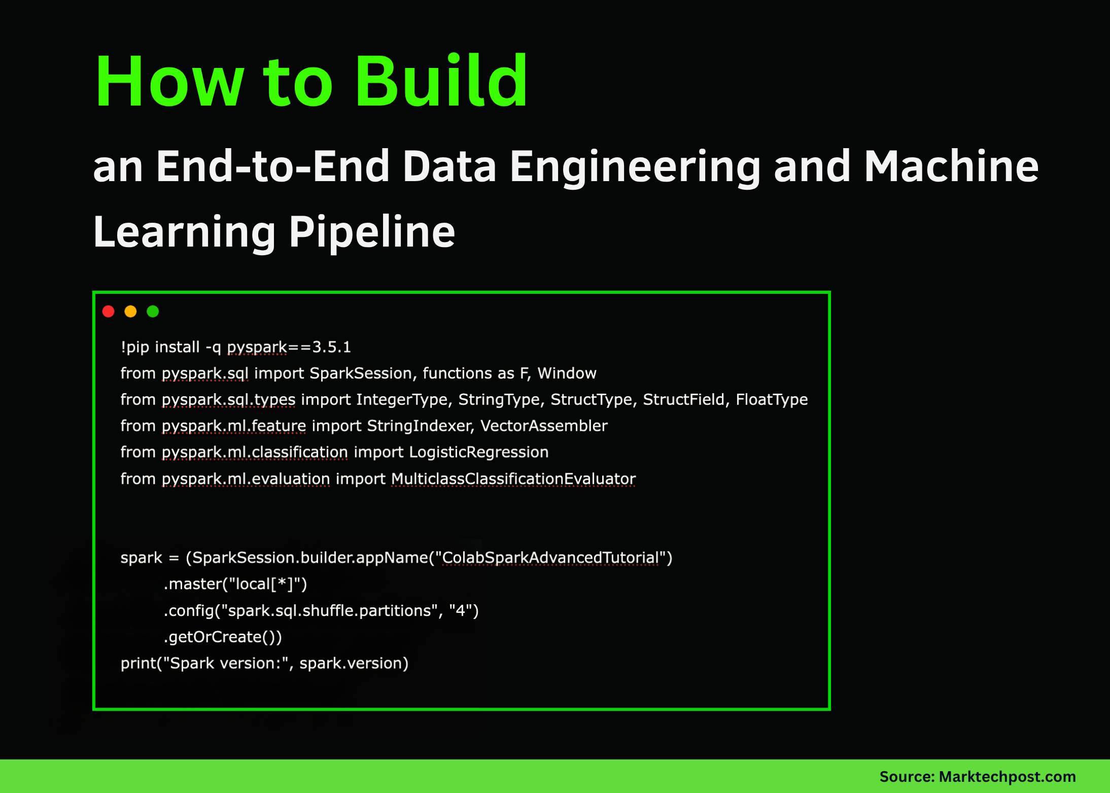
In this tutorial, we explore how to harness Apache Spark’s techniques using PySpark directly in Google Colab. We begin by setting up a local Spark session, then progressively move through transformations, SQL queries, joins, and window functions. We also build and evaluate a simple machine-learning model to predict user subscription types and finally demonstrate how to save and reload Parquet files. Also, we experience how Spark’s distributed data-processing capabilities can be leveraged for analytics and ML workflows even in a single-node Colab environment. Check out the FULL CODES here.
!pip install -q pyspark==3.5.1
from pyspark.sql import SparkSession, functions as F, Window
from pyspark.sql.types import IntegerType, StringType, StructType, StructField, FloatType
from pyspark.ml.feature import StringIndexer, VectorAssembler
from pyspark.ml.classification import LogisticRegression
from pyspark.ml.evaluation import MulticlassClassificationEvaluator


spark = (SparkSession.builder.appName("ColabSparkAdvancedTutorial")
        .master("local[*]")
        .config("spark.sql.shuffle.partitions", "4")
        .getOrCreate())
print("Spark version:", spark.version)


data = [
   (1, "Alice", "IN", "2025-10-01", 56000.0, "premium"),
   (2, "Bob", "US", "2025-10-03", 43000.0, "standard"),
   (3, "Carlos", "IN", "2025-09-27", 72000.0, "premium"),
   (4, "Diana", "UK", "2025-09-30", 39000.0, "standard"),
   (5, "Esha", "IN", "2025-10-02", 85000.0, "premium"),
   (6, "Farid", "AE", "2025-10-02", 31000.0, "basic"),
   (7, "Gita", "IN", "2025-09-29", 46000.0, "standard"),
   (8, "Hassan", "PK", "2025-10-01", 52000.0, "premium"),
]
schema = StructType([
   StructField("id", IntegerType(), False),
   StructField("name", StringType(), True),
   StructField("country", StringType(), True),
   StructField("signup_date", StringType(), True),
   StructField("income", FloatType(), True),
   StructField("plan", StringType(), True),
])
df = spark.createDataFrame(data, schema)
df.show()
We begin by setting up PySpark, initializing the Spark session, and preparing our dataset. We create a structured DataFrame containing user information, including country, income, and plan type. This forms the foundation for all transformations and analyses that follow. Check out the FULL CODES here.
df2 = (df.withColumn("signup_ts", F.to_timestamp("signup_date"))
        .withColumn("year", F.year("signup_ts"))
        .withColumn("month", F.month("signup_ts"))
        .withColumn("is_india", (F.col("country") == "IN").cast("int")))
df2.show()


df2.createOrReplaceTempView("users")
spark.sql("""
SELECT country, COUNT(*) AS cnt, AVG(income) AS avg_income
FROM users
GROUP BY country
ORDER BY cnt DESC
""").show()


w = Window.partitionBy("country").orderBy(F.col("income").desc())
df_ranked = df2.withColumn("income_rank_in_country", F.rank().over(w))
df_ranked.show()


def plan_priority(plan):
   if plan == "premium": return 3
   if plan == "standard": return 2
   if plan == "basic": return 1
   return 0
plan_priority_udf = F.udf(plan_priority, IntegerType())
df_udf = df_ranked.withColumn("plan_priority", plan_priority_udf(F.col("plan")))
df_udf.show()
We now perform various data transformations, add new columns, and register the DataFrame as a SQL table. We explore Spark SQL for aggregation and apply window functions to rank users by income. We also introduce a user-defined function (UDF) to assign priority levels to subscription plans. Check out the FULL CODES here.
country_data = [
   ("IN", "Asia", 1.42), ("US", "North America", 0.33),
   ("UK", "Europe", 0.07), ("AE", "Asia", 0.01), ("PK", "Asia", 0.24),
]
country_schema = StructType([
   StructField("country", StringType(), True),
   StructField("region", StringType(), True),
   StructField("population_bn", FloatType(), True),
])
country_df = spark.createDataFrame(country_data, country_schema)


joined = df_udf.alias("u").join(country_df.alias("c"), on="country", how="left")
joined.show()


region_stats = (joined.groupBy("region", "plan")
               .agg(F.count("*").alias("users"),
                    F.round(F.avg("income"), 2).alias("avg_income"))
               .orderBy("region", "plan"))
region_stats.show()
We enrich our user dataset by joining it with country-level metadata that includes region and population. We then compute analytical summaries such as average income and user counts by region and plan type. This step demonstrates how Spark simplifies the seamless combination and aggregation of large datasets. Check out the FULL CODES here.
ml_df = joined.withColumn("label", (F.col("plan") == "premium").cast("int")).na.drop()
country_indexer = StringIndexer(inputCol="country", outputCol="country_idx", handleInvalid="keep")
country_fitted = country_indexer.fit(ml_df)
ml_df2 = country_fitted.transform(ml_df)


assembler = VectorAssembler(inputCols=["income", "country_idx", "plan_priority"], outputCol="features")
ml_final = assembler.transform(ml_df2)
train_df, test_df = ml_final.randomSplit([0.7, 0.3], seed=42)


lr = LogisticRegression(featuresCol="features", labelCol="label", maxIter=20)
lr_model = lr.fit(train_df)
preds = lr_model.transform(test_df)
preds.select("name", "country", "income", "plan", "label", "prediction", "probability").show(truncate=False)


evaluator = MulticlassClassificationEvaluator(labelCol="label", predictionCol="prediction", metricName="accuracy")
acc = evaluator.evaluate(preds)
print("Classification accuracy:", acc)
We move into machine learning by preparing data for model training and feature engineering. We index categorical columns, assemble features, and train a logistic regression model to predict premium users. We then evaluate its accuracy, showcasing how Spark MLlib integrates easily into the data workflow. Check out the FULL CODES here.
output_path = "/content/spark_users_parquet"
joined.write.mode("overwrite").parquet(output_path)
parquet_df = spark.read.parquet(output_path)
print("Parquet reloaded:")
parquet_df.show()


recent = spark.sql("""
SELECT name, country, income, signup_ts
FROM users
WHERE signup_ts >= '2025-10-01'
ORDER BY signup_ts DESC
""")
recent.show()


recent.explain()
spark.stop()
We conclude by writing the processed data to Parquet format and reading it back into Spark for verification. We run a SQL query to extract recent signups and inspect the query plan for optimization insights. Finally, we gracefully stop the Spark session to complete our workflow.
In conclusion, we gain a practical understanding of how PySpark unifies data engineering and machine learning tasks within a single scalable framework. We witness how simple DataFrame transformations evolve into SQL analytics, feature engineering, and predictive modeling, all while staying within Google Colab. By experimenting with these concepts, we strengthen our ability to prototype and deploy Spark-based data solutions efficiently in both local and distributed setups.
Check out the FULL CODES here. Feel free to check out our GitHub Page for Tutorials, Codes and Notebooks. Also, feel free to follow us on Twitter and don’t forget to join our 100k+ ML SubReddit and Subscribe to our Newsletter. Wait! are you on telegram? now you can join us on telegram as well.
The post How to Build an End-to-End Data Engineering and Machine Learning Pipeline with Apache Spark and PySpark appeared first on MarkTechPost.


