
In this tutorial, we explore how to build and train an advanced neural network using JAX, Flax, and Optax in an efficient and modular way. We begin by designing a deep architecture that integrates residual connections and self-attention mechanisms for expressive feature learning. As we progress, we implement sophisticated optimization strategies with learning rate scheduling, gradient clipping, and adaptive weight decay. Throughout the process, we leverage JAX transformations such as jit, grad, and vmap to accelerate computation and ensure smooth training performance across devices. Check out the FULL CODES here.
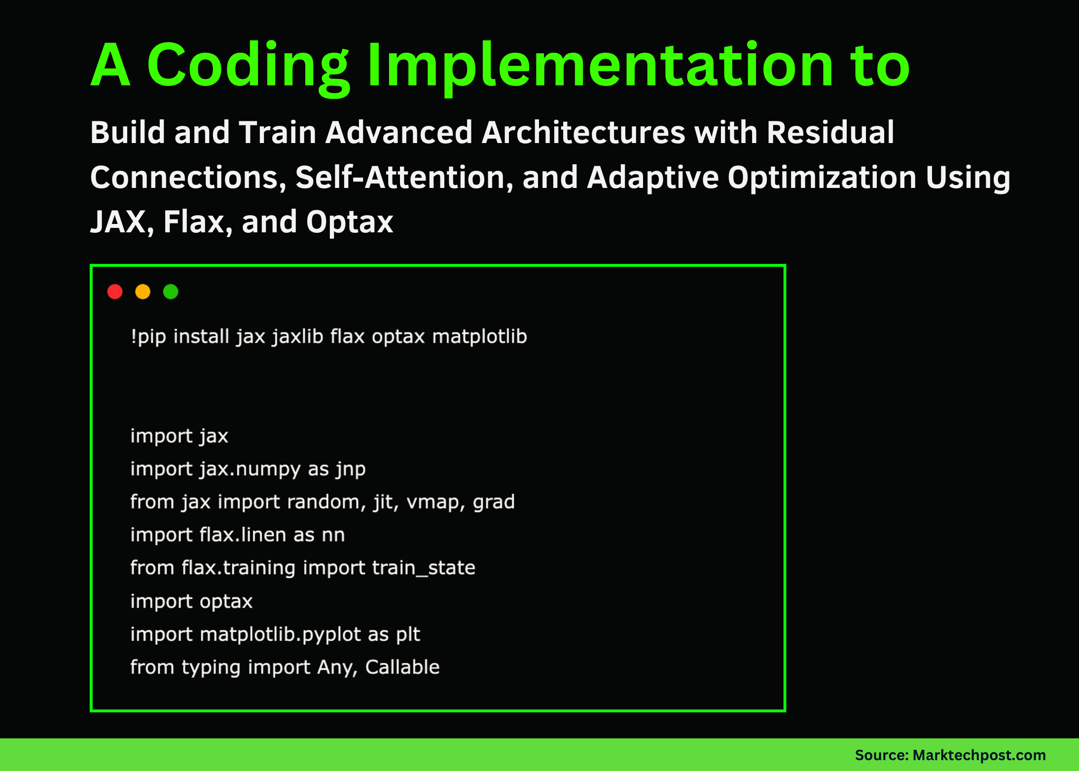
!pip install jax jaxlib flax optax matplotlib


import jax
import jax.numpy as jnp
from jax import random, jit, vmap, grad
import flax.linen as nn
from flax.training import train_state
import optax
import matplotlib.pyplot as plt
from typing import Any, Callable


print(f"JAX version: {jax.__version__}")
print(f"Devices: {jax.devices()}")
We begin by installing and importing JAX, Flax, and Optax, along with essential utilities for numerical operations and visualization. We check our device setup to ensure that JAX is running efficiently on available hardware. This setup forms the foundation for the entire training pipeline. Check out the FULL CODES here.
class SelfAttention(nn.Module):
   num_heads: int
   dim: int
   @nn.compact
   def __call__(self, x):
       B, L, D = x.shape
       head_dim = D // self.num_heads
       qkv = nn.Dense(3 * D)(x)
       qkv = qkv.reshape(B, L, 3, self.num_heads, head_dim)
       q, k, v = jnp.split(qkv, 3, axis=2)
       q, k, v = q.squeeze(2), k.squeeze(2), v.squeeze(2)
       attn_scores = jnp.einsum('bhqd,bhkd->bhqk', q, k) / jnp.sqrt(head_dim)
       attn_weights = jax.nn.softmax(attn_scores, axis=-1)
       attn_output = jnp.einsum('bhqk,bhvd->bhqd', attn_weights, v)
       attn_output = attn_output.reshape(B, L, D)
       return nn.Dense(D)(attn_output)


class ResidualBlock(nn.Module):
   features: int
   @nn.compact
   def __call__(self, x, training: bool = True):
       residual = x
       x = nn.Conv(self.features, (3, 3), padding='SAME')(x)
       x = nn.BatchNorm(use_running_average=not training)(x)
       x = nn.relu(x)
       x = nn.Conv(self.features, (3, 3), padding='SAME')(x)
       x = nn.BatchNorm(use_running_average=not training)(x)
       if residual.shape[-1] != self.features:
           residual = nn.Conv(self.features, (1, 1))(residual)
       return nn.relu(x + residual)


class AdvancedCNN(nn.Module):
   num_classes: int = 10
   @nn.compact
   def __call__(self, x, training: bool = True):
       x = nn.Conv(32, (3, 3), padding='SAME')(x)
       x = nn.relu(x)
       x = ResidualBlock(64)(x, training)
       x = ResidualBlock(64)(x, training)
       x = nn.max_pool(x, (2, 2), strides=(2, 2))
       x = ResidualBlock(128)(x, training)
       x = ResidualBlock(128)(x, training)
       x = jnp.mean(x, axis=(1, 2))
       x = x[:, None, :]
       x = SelfAttention(num_heads=4, dim=128)(x)
       x = x.squeeze(1)
       x = nn.Dense(256)(x)
       x = nn.relu(x)
       x = nn.Dropout(0.5, deterministic=not training)(x)
       x = nn.Dense(self.num_classes)(x)
       return x
We define a deep neural network that combines residual blocks and a self-attention mechanism for enhanced feature learning. We construct the layers modularly, ensuring that the model can capture both spatial and contextual relationships. This design enables the network to generalize effectively across various types of input data. Check out the FULL CODES here.
class TrainState(train_state.TrainState):
   batch_stats: Any


def create_learning_rate_schedule(base_lr: float = 1e-3, warmup_steps: int = 100, decay_steps: int = 1000) -> optax.Schedule:
   warmup_fn = optax.linear_schedule(init_value=0.0, end_value=base_lr, transition_steps=warmup_steps)
   decay_fn = optax.cosine_decay_schedule(init_value=base_lr, decay_steps=decay_steps, alpha=0.1)
   return optax.join_schedules(schedules=[warmup_fn, decay_fn], boundaries=[warmup_steps])


def create_optimizer(learning_rate_schedule: optax.Schedule) -> optax.GradientTransformation:
   return optax.chain(optax.clip_by_global_norm(1.0), optax.adamw(learning_rate=learning_rate_schedule, weight_decay=1e-4))
We create a custom training state that tracks model parameters and batch statistics. We also define a learning rate schedule with warmup and cosine decay, paired with an AdamW optimizer that includes gradient clipping and weight decay. This combination ensures stable and adaptive training. Check out the FULL CODES here.
@jit
def compute_metrics(logits, labels):
   loss = optax.softmax_cross_entropy_with_integer_labels(logits, labels).mean()
   accuracy = jnp.mean(jnp.argmax(logits, -1) == labels)
   return {'loss': loss, 'accuracy': accuracy}


def create_train_state(rng, model, input_shape, learning_rate_schedule):
   variables = model.init(rng, jnp.ones(input_shape), training=False)
   params = variables['params']
   batch_stats = variables.get('batch_stats', {})
   tx = create_optimizer(learning_rate_schedule)
   return TrainState.create(apply_fn=model.apply, params=params, tx=tx, batch_stats=batch_stats)


@jit
def train_step(state, batch, dropout_rng):
   images, labels = batch
   def loss_fn(params):
       variables = {'params': params, 'batch_stats': state.batch_stats}
       logits, new_model_state = state.apply_fn(variables, images, training=True, mutable=['batch_stats'], rngs={'dropout': dropout_rng})
       loss = optax.softmax_cross_entropy_with_integer_labels(logits, labels).mean()
       return loss, (logits, new_model_state)
   grad_fn = jax.value_and_grad(loss_fn, has_aux=True)
   (loss, (logits, new_model_state)), grads = grad_fn(state.params)
   state = state.apply_gradients(grads=grads, batch_stats=new_model_state['batch_stats'])
   metrics = compute_metrics(logits, labels)
   return state, metrics


@jit
def eval_step(state, batch):
   images, labels = batch
   variables = {'params': state.params, 'batch_stats': state.batch_stats}
   logits = state.apply_fn(variables, images, training=False)
   return compute_metrics(logits, labels)
We implement JIT-compiled training and evaluation functions to achieve efficient execution. The training step computes gradients, updates parameters, and dynamically maintains batch statistics. We also define evaluation metrics that help us monitor loss and accuracy throughout the training process. Check out the FULL CODES here.
def generate_synthetic_data(rng, num_samples=1000, img_size=32):
   rng_x, rng_y = random.split(rng)
   images = random.normal(rng_x, (num_samples, img_size, img_size, 3))
   labels = random.randint(rng_y, (num_samples,), 0, 10)
   return images, labels


def create_batches(images, labels, batch_size=32):
   num_batches = len(images) // batch_size
   for i in range(num_batches):
       idx = slice(i * batch_size, (i + 1) * batch_size)
       yield images[idx], labels[idx]
We generate synthetic data to simulate an image classification task, enabling us to train the model without relying on external datasets. We then batch the data efficiently for iterative updates. This approach allows us to test the full pipeline quickly and verify that all components function correctly. Check out the FULL CODES here.
def train_model(num_epochs=5, batch_size=32):
   rng = random.PRNGKey(0)
   rng, data_rng, model_rng = random.split(rng, 3)
   train_images, train_labels = generate_synthetic_data(data_rng, num_samples=1000)
   test_images, test_labels = generate_synthetic_data(data_rng, num_samples=200)
   model = AdvancedCNN(num_classes=10)
   lr_schedule = create_learning_rate_schedule(base_lr=1e-3, warmup_steps=50, decay_steps=500)
   state = create_train_state(model_rng, model, (1, 32, 32, 3), lr_schedule)
   history = {'train_loss': [], 'train_acc': [], 'test_acc': []}
   print("Starting training...")
   for epoch in range(num_epochs):
       train_metrics = []
       for batch in create_batches(train_images, train_labels, batch_size):
           rng, dropout_rng = random.split(rng)
           state, metrics = train_step(state, batch, dropout_rng)
           train_metrics.append(metrics)
       train_loss = jnp.mean(jnp.array([m['loss'] for m in train_metrics]))
       train_acc = jnp.mean(jnp.array([m['accuracy'] for m in train_metrics]))
       test_metrics = [eval_step(state, batch) for batch in create_batches(test_images, test_labels, batch_size)]
       test_acc = jnp.mean(jnp.array([m['accuracy'] for m in test_metrics]))
       history['train_loss'].append(float(train_loss))
       history['train_acc'].append(float(train_acc))
       history['test_acc'].append(float(test_acc))
       print(f"Epoch {epoch + 1}/{num_epochs}: Loss: {train_loss:.4f}, Train Acc: {train_acc:.4f}, Test Acc: {test_acc:.4f}")
   return history, state


history, trained_state = train_model(num_epochs=5)


fig, (ax1, ax2) = plt.subplots(1, 2, figsize=(12, 4))
ax1.plot(history['train_loss'], label='Train Loss')
ax1.set_xlabel('Epoch'); ax1.set_ylabel('Loss'); ax1.set_title('Training Loss'); ax1.legend(); ax1.grid(True)
ax2.plot(history['train_acc'], label='Train Accuracy')
ax2.plot(history['test_acc'], label='Test Accuracy')
ax2.set_xlabel('Epoch'); ax2.set_ylabel('Accuracy'); ax2.set_title('Model Accuracy'); ax2.legend(); ax2.grid(True)
plt.tight_layout(); plt.show()


print("n Tutorial complete! This covers:")
print("- Custom Flax modules (ResNet blocks, Self-Attention)")
print("- Advanced Optax optimizers (AdamW with gradient clipping)")
print("- Learning rate schedules (warmup + cosine decay)")
print("- JAX transformations (@jit for performance)")
print("- Proper state management (batch normalization statistics)")
print("- Complete training pipeline with evaluation")
Tutorial complete! This covers:")
print("- Custom Flax modules (ResNet blocks, Self-Attention)")
print("- Advanced Optax optimizers (AdamW with gradient clipping)")
print("- Learning rate schedules (warmup + cosine decay)")
print("- JAX transformations (@jit for performance)")
print("- Proper state management (batch normalization statistics)")
print("- Complete training pipeline with evaluation")We bring all components together to train the model over several epochs, track performance metrics, and visualize the trends in loss and accuracy. We monitor the model’s learning progress and validate its performance on test data. Ultimately, we confirm the stability and effectiveness of our JAX-based training workflow.
In conclusion, we implemented a comprehensive training pipeline utilizing JAX, Flax, and Optax, which demonstrates both flexibility and computational efficiency. We observed how custom architectures, advanced optimization strategies, and precise state management can come together to form a high-performance deep learning workflow. Through this exercise, we gain a deeper understanding of how to structure scalable experiments in JAX and prepare ourselves to adapt these techniques to real-world machine learning research and production tasks.
Check out the FULL CODES here. Feel free to check out our GitHub Page for Tutorials, Codes and Notebooks. Also, feel free to follow us on Twitter and don’t forget to join our 100k+ ML SubReddit and Subscribe to our Newsletter. Wait! are you on telegram? now you can join us on telegram as well.
The post A Coding Implementation to Build and Train Advanced Architectures with Residual Connections, Self-Attention, and Adaptive Optimization Using JAX, Flax, and Optax appeared first on MarkTechPost.


